EDA of USA National Weather Service Storm Data
EDA of U.S. National Oceanic and Atmospheric Administration’s storm database (part of Reproducible Research Analysis by Johns Hopkins University)
This assignment was part of the Johns Hopkins Coursera module on Reproducible Research as part of the Data Sciene Specialization.
Source code available on GitHub
National Weather Service Storm Data Documentation
National Climatic Data Center Storm Events FAQ
Synopsis
The purpose of this analysis is to answer two questions:
- Across the United States, which types of events are most harmful with respect to population health?
- Across the United States, which types of events have the greatest economic consequences?
For the first question, we need to quantify harmful considering the data we have at hands. Two variables can be seen as good candidates:
- injuries
- casualties
To simplify our analysis we will consider that both variables account for the same degree of harm to population health, and that the count of injuries and casualties is a good indicator.
For the second question, we need to quantify economic consequences considering the data we have at hands. Two variables can be seen as good candidates (associated with their explanoratory variables):
- propdmg
- cropdmg
These variables summarize estimates of damage in dollars amount, and we will consider the sum of these to be a good indicator for our purpose.
Data Processing
library(dplyr)
library(tidyr)
library(forcats)
library(ggplot2)
library(knitr)
Loading data
URL = "https://d396qusza40orc.cloudfront.net/repdata%2Fdata%2FStormData.csv.bz2"
FILE = "stormdata.csv.bz2"
if (!file.exists(FILE)) {
  download.file(URL, FILE, method="libcurl")
}

storm.data <- read.csv(FILE)
colnames(storm.data) <- make.names(casefold(colnames(storm.data), upper = FALSE), unique=TRUE, allow_ = FALSE)
Glimpse at data
head(storm.data)
##   state..           bgn.date bgn.time time.zone county countyname state
## 1       1  4/18/1950 0:00:00     0130       CST     97     MOBILE    AL
## 2       1  4/18/1950 0:00:00     0145       CST      3    BALDWIN    AL
## 3       1  2/20/1951 0:00:00     1600       CST     57    FAYETTE    AL
## 4       1   6/8/1951 0:00:00     0900       CST     89    MADISON    AL
## 5       1 11/15/1951 0:00:00     1500       CST     43    CULLMAN    AL
## 6       1 11/15/1951 0:00:00     2000       CST     77 LAUDERDALE    AL
##    evtype bgn.range bgn.azi bgn.locati end.date end.time county.end
## 1 TORNADO         0                                               0
## 2 TORNADO         0                                               0
## 3 TORNADO         0                                               0
## 4 TORNADO         0                                               0
## 5 TORNADO         0                                               0
## 6 TORNADO         0                                               0
##   countyendn end.range end.azi end.locati length width f mag fatalities
## 1         NA         0                      14.0   100 3   0          0
## 2         NA         0                       2.0   150 2   0          0
## 3         NA         0                       0.1   123 2   0          0
## 4         NA         0                       0.0   100 2   0          0
## 5         NA         0                       0.0   150 2   0          0
## 6         NA         0                       1.5   177 2   0          0
##   injuries propdmg propdmgexp cropdmg cropdmgexp wfo stateoffic zonenames
## 1       15    25.0          K       0
## 2        0     2.5          K       0
## 3        2    25.0          K       0
## 4        2     2.5          K       0
## 5        2     2.5          K       0
## 6        6     2.5          K       0
##   latitude longitude latitude.e longitude. remarks refnum
## 1     3040      8812       3051       8806              1
## 2     3042      8755          0          0              2
## 3     3340      8742          0          0              3
## 4     3458      8626          0          0              4
## 5     3412      8642          0          0              5
## 6     3450      8748          0          0              6
str(storm.data)
## 'data.frame':    902297 obs. of  37 variables:
##  $ state..   : num  1 1 1 1 1 1 1 1 1 1 ...
##  $ bgn.date  : Factor w/ 16335 levels "1/1/1966 0:00:00",..: 6523 6523 4242 11116 2224 2224 2260 383 3980 3980 ...
##  $ bgn.time  : Factor w/ 3608 levels "00:00:00 AM",..: 272 287 2705 1683 2584 3186 242 1683 3186 3186 ...
##  $ time.zone : Factor w/ 22 levels "ADT","AKS","AST",..: 7 7 7 7 7 7 7 7 7 7 ...
##  $ county    : num  97 3 57 89 43 77 9 123 125 57 ...
##  $ countyname: Factor w/ 29601 levels "","5NM E OF MACKINAC BRIDGE TO PRESQUE ISLE LT MI",..: 13513 1873 4598 10592 4372 10094 1973 23873 24418 4598 ...
##  $ state     : Factor w/ 72 levels "AK","AL","AM",..: 2 2 2 2 2 2 2 2 2 2 ...
##  $ evtype    : Factor w/ 985 levels "   HIGH SURF ADVISORY",..: 834 834 834 834 834 834 834 834 834 834 ...
##  $ bgn.range : num  0 0 0 0 0 0 0 0 0 0 ...
##  $ bgn.azi   : Factor w/ 35 levels "","  N"," NW",..: 1 1 1 1 1 1 1 1 1 1 ...
##  $ bgn.locati: Factor w/ 54429 levels "","- 1 N Albion",..: 1 1 1 1 1 1 1 1 1 1 ...
##  $ end.date  : Factor w/ 6663 levels "","1/1/1993 0:00:00",..: 1 1 1 1 1 1 1 1 1 1 ...
##  $ end.time  : Factor w/ 3647 levels ""," 0900CST",..: 1 1 1 1 1 1 1 1 1 1 ...
##  $ county.end: num  0 0 0 0 0 0 0 0 0 0 ...
##  $ countyendn: logi  NA NA NA NA NA NA ...
##  $ end.range : num  0 0 0 0 0 0 0 0 0 0 ...
##  $ end.azi   : Factor w/ 24 levels "","E","ENE","ESE",..: 1 1 1 1 1 1 1 1 1 1 ...
##  $ end.locati: Factor w/ 34506 levels "","- .5 NNW",..: 1 1 1 1 1 1 1 1 1 1 ...
##  $ length    : num  14 2 0.1 0 0 1.5 1.5 0 3.3 2.3 ...
##  $ width     : num  100 150 123 100 150 177 33 33 100 100 ...
##  $ f         : int  3 2 2 2 2 2 2 1 3 3 ...
##  $ mag       : num  0 0 0 0 0 0 0 0 0 0 ...
##  $ fatalities: num  0 0 0 0 0 0 0 0 1 0 ...
##  $ injuries  : num  15 0 2 2 2 6 1 0 14 0 ...
##  $ propdmg   : num  25 2.5 25 2.5 2.5 2.5 2.5 2.5 25 25 ...
##  $ propdmgexp: Factor w/ 19 levels "","-","?","+",..: 17 17 17 17 17 17 17 17 17 17 ...
##  $ cropdmg   : num  0 0 0 0 0 0 0 0 0 0 ...
##  $ cropdmgexp: Factor w/ 9 levels "","?","0","2",..: 1 1 1 1 1 1 1 1 1 1 ...
##  $ wfo       : Factor w/ 542 levels ""," CI","$AC",..: 1 1 1 1 1 1 1 1 1 1 ...
##  $ stateoffic: Factor w/ 250 levels "","ALABAMA, Central",..: 1 1 1 1 1 1 1 1 1 1 ...
##  $ zonenames : Factor w/ 25112 levels "","                                                                                                               "| __truncated__,..: 1 1 1 1 1 1 1 1 1 1 ...
##  $ latitude  : num  3040 3042 3340 3458 3412 ...
##  $ longitude : num  8812 8755 8742 8626 8642 ...
##  $ latitude.e: num  3051 0 0 0 0 ...
##  $ longitude.: num  8806 0 0 0 0 ...
##  $ remarks   : Factor w/ 436781 levels "","-2 at Deer Park\n",..: 1 1 1 1 1 1 1 1 1 1 ...
##  $ refnum    : num  1 2 3 4 5 6 7 8 9 10 ...
1. Across the United States, which types of events are most harmful with respect to population health?
For first question we will use the injuries and fatalities columns which do not appear to have any specific or impacting issues.
summary(storm.data[,c("injuries", "fatalities")])
##     injuries           fatalities
##  Min.   :   0.0000   Min.   :  0.0000
##  1st Qu.:   0.0000   1st Qu.:  0.0000
##  Median :   0.0000   Median :  0.0000
##  Mean   :   0.1557   Mean   :  0.0168
##  3rd Qu.:   0.0000   3rd Qu.:  0.0000
##  Max.   :1700.0000   Max.   :583.0000
sum(is.na(storm.data[,c("injuries", "fatalities")]))
## [1] 0
We take the assumption that the number of injuries and fatalities characterizes the harm to population health in equal weight. Thus we look for the events for which the cumulated number of injuries and fatalities are the highest.
Let’s summarize data accordingly:
data.1 <- storm.data %>% group_by(evtype) %>%
  summarise_at(vars(fatalities, injuries), sum) %>%
  top_n(5, fatalities + injuries) %>%
  mutate(evtype = fct_drop(evtype)) %>%
  mutate(evtype = fct_reorder(evtype, fatalities + injuries, .desc = TRUE)) %>%
  pivot_longer(c(fatalities, injuries), names_to="casualty.type", values_to ="casualties")
2. Across the United States, which types of events have the greatest economic consequences?
For the second question we will use the propdmg, prodmgexp, cropdmg and cropdmgexp columns (we could drop the crop variables considering the values).
summary(storm.data$propdmgexp)
##             -      ?      +      0      1      2      3      4      5
## 465934      1      8      5    216     25     13      4      4     28
##      6      7      8      B      h      H      K      m      M
##      4      5      1     40      1      6 424665      7  11330
non.char.levels <- levels(storm.data$propdmgexp)[!grepl("[A-z]", levels(storm.data$propdmgexp))]
char.levels <- levels(storm.data$propdmgexp)[grepl("[A-z]", levels(storm.data$propdmgexp))]

storm.data %>% mutate(dmg.level = propdmgexp %in% non.char.levels) %>%
  group_by(dmg.level) %>%
  summarise(total = sum(propdmg))
## # A tibble: 2 x 2
##   dmg.level     total
##   <lgl>         <dbl>
## 1 FALSE     10876328.
## 2 TRUE          8172.
# Similar work for the cropdmg exp
storm.data %>% mutate(dmg.level = cropdmgexp %in% non.char.levels) %>%
  group_by(dmg.level) %>%
  summarise(total = sum(cropdmg))
## # A tibble: 2 x 2
##   dmg.level    total
##   <lgl>        <dbl>
## 1 FALSE     1377556.
## 2 TRUE          271
There is not much information on the prodmgexp and cropdmgexp
variables.
When we look at those variables, we can find what looks like standard
M/K/B SI units (in addition to H). We will chose to ignore levels that
are not one of B, h, H, K, m, M, considering the lack of information
and the fact that the associated amount are limited compared to the
rest.
Let’s summarize data accordingly:
data.2 <- storm.data %>% group_by(evtype) %>%
  filter(propdmgexp %in% char.levels | cropdmgexp %in% char.levels) %>%
  mutate(propdmgexp = casefold(propdmgexp, upper=TRUE), cropdmgexp = casefold(cropdmgexp, upper=TRUE)) %>%
  mutate(propdmg = case_when(
    propdmgexp == "H" ~ propdmg*100,
    propdmgexp == "K" ~ propdmg*1000,
    propdmgexp == "M" ~ propdmg*1000000,
    propdmgexp == "B" ~ propdmg*1000000000,
  )) %>%
  mutate(cropdmg = case_when(
    cropdmgexp == "H" ~ cropdmg*100,
    cropdmgexp == "K" ~ cropdmg*1000,
    cropdmgexp == "M" ~ cropdmg*1000000,
    cropdmgexp == "B" ~ cropdmg*1000000000,
  )) %>%
  summarise_at(vars(propdmg, cropdmg), sum) %>%
  top_n(5, propdmg + cropdmg) %>%
  mutate(evtype = fct_drop(evtype)) %>%
  mutate(evtype = fct_reorder(evtype, propdmg + cropdmg, .desc = TRUE)) %>%
  pivot_longer(c(propdmg, cropdmg), names_to="damage.type", values_to ="amount")
Results
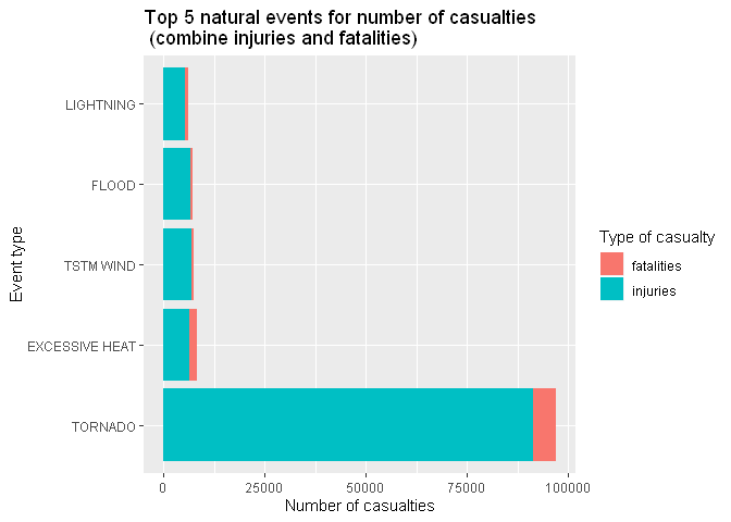
1. Across the United States, which types of events are most harmful with respect to population health?
we plot the top 5 type of events considering the number of casualties.
We can see that the tornadoes are #1 by order of magnitudes.
g.1 <- ggplot(data.1, aes(evtype, casualties, fill=casualty.type))
g.1 <- g.1 + geom_col(position="stack")
g.1 <- g.1 + labs(title="Top 5 natural events for number of casualties \n (combine injuries and fatalities)", x="Event type", y="Number of casualties")
g.1 <- g.1 + scale_fill_discrete(name="Type of casualty")
g.1 <- g.1 + coord_flip()
g.1
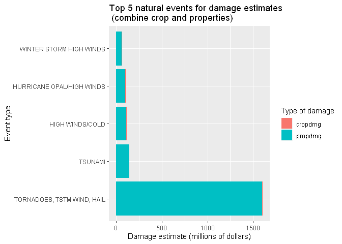
2. Across the United States, which types of events have the greatest economic consequences?
we plot the top 5 type of events considering the amount of damages.
We can see again that the tornadoes are #1 by order of magnitudes.
g.2 <- ggplot(data.2, aes(evtype, amount/1000000, fill=damage.type))
g.2 <- g.2 + geom_col(position="stack")
g.2 <- g.2 + labs(title="Top 5 natural events for damage estimates \n (combine crop and properties)", x="Event type", y="Damage estimate (millions of dollars)")
g.2 <- g.2 + scale_fill_discrete(name="Type of damage")
g.2 <- g.2 + coord_flip()
g.2