EDA of activity monitoring data

Activity monitoring (part of Reproducible Research module by Johns Hopkins University)

This assignment was part of the Johns Hopkins Coursera module on Reproducible Research as part of the Data Sciene Specialization.

Full code can be found on GitHub.

Loading and preprocessing the data

The variables included in this dataset are:

• steps: Number of steps taking in a 5-minute interval (missing values are coded as NA)

• date: The date on which the measurement was taken in YYYY-MM-DD format

• interval: Identifier for the 5-minute interval in which measurement was taken

The dataset is stored in a comma-separated-value (CSV) file and there are a total of 17,568 observations in this dataset.

Loading the data:

if (!file.exists("activity.csv")){
  unzip("activity.zip")
}
data <- read.csv("activity.csv", na.strings = "NA", colClasses = c("integer", "character", "integer"))
data$date <- as.Date(data$date, format="%Y-%m-%d")

Checking the data:

str(data)

## 'data.frame':	17568 obs. of  3 variables:
##  $ steps   : int  NA NA NA NA NA NA NA NA NA NA ...
##  $ date    : Date, format: "2012-10-01" "2012-10-01" ...
##  $ interval: int  0 5 10 15 20 25 30 35 40 45 ...

summary(data)

##      steps             date               interval     
##  Min.   :  0.00   Min.   :2012-10-01   Min.   :   0.0  
##  1st Qu.:  0.00   1st Qu.:2012-10-16   1st Qu.: 588.8  
##  Median :  0.00   Median :2012-10-31   Median :1177.5  
##  Mean   : 37.38   Mean   :2012-10-31   Mean   :1177.5  
##  3rd Qu.: 12.00   3rd Qu.:2012-11-15   3rd Qu.:1766.2  
##  Max.   :806.00   Max.   :2012-11-30   Max.   :2355.0  
##  NA's   :2304

head(data)

##   steps       date interval
## 1    NA 2012-10-01        0
## 2    NA 2012-10-01        5
## 3    NA 2012-10-01       10
## 4    NA 2012-10-01       15
## 5    NA 2012-10-01       20
## 6    NA 2012-10-01       25

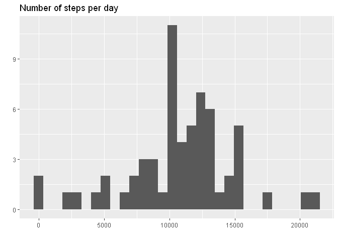
What is mean total number of steps taken per day?

For this part of the assignment, you can ignore the missing values in the dataset.

Summarizing the data:

total_steps <- data %>% group_by(date) %>%
  summarise(total = sum(steps, na.rm = TRUE))

g <- ggplot(total_steps, aes(total))
g <- g + geom_histogram()
g <- g + labs(title="Number of steps per day", y="", x="")
g

## `stat_bin()` using `bins = 30`. Pick better value with `binwidth`.

mean <- mean(total_steps$total, na.rm = TRUE)
mean

## [1] 9354.23

The mean total number of steps per day is: 9354.23

median <- median(total_steps$total, na.rm = TRUE)
median

## [1] 10395

The median total number of steps per day is: 10395

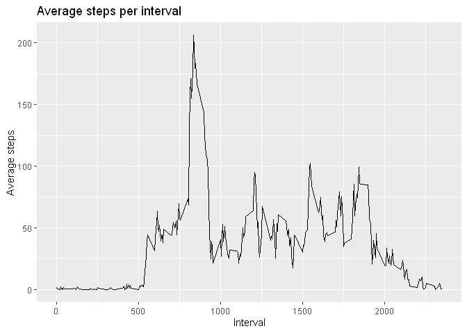
What is the average daily activity pattern?

Summarizing the data:

steps_interval <- data %>% group_by(interval) %>%
  summarise(mean = mean(steps, na.rm = TRUE))

g <- ggplot(steps_interval, aes(interval, mean))
g <- g + geom_line()
g <- g + labs(title="Average steps per interval", y="Average steps", x="Interval")
g

ix <- which.max(steps_interval$mean)
interval <- steps_interval[[ix, "interval"]]
val <- steps_interval[[ix, "mean"]]

The interval with max mean number of steps is 835 with a mean number of steps of 206.17.

h <- floor(interval/60)
m <- interval%%60

Supposing the interval starts at 00:00 of each day, this interval corresponds to 13:55.

Imputing missing values

Total number of missing values:

apply(is.na(data), 2, sum)

##    steps     date interval 
##     2304        0        0

We will fill in the missing steps values with the mean for the specific day and interval.

First we compute the mean for each interval and day of the week.

data <- data %>% mutate(weekday = as.factor(as.POSIXlt(date)$wday))
fill_val <- data %>% group_by(weekday, interval) %>%
  summarise(mean = mean(steps, na.rm = TRUE))

Imputing missing data.

data_nna <- data

for (row in 1:nrow(data_nna)) {
  if(is.na(data_nna[row, "steps"])) {
    wd <- data_nna[row, "weekday"]
    interval <- data[row, "interval"]
    data_nna[row, "steps"] <- fill_val[fill_val$weekday==wd & fill_val$interval==interval, "mean"]
  }
}

apply(is.na(data_nna), 2, sum)

##    steps     date interval  weekday 
##        0        0        0        0

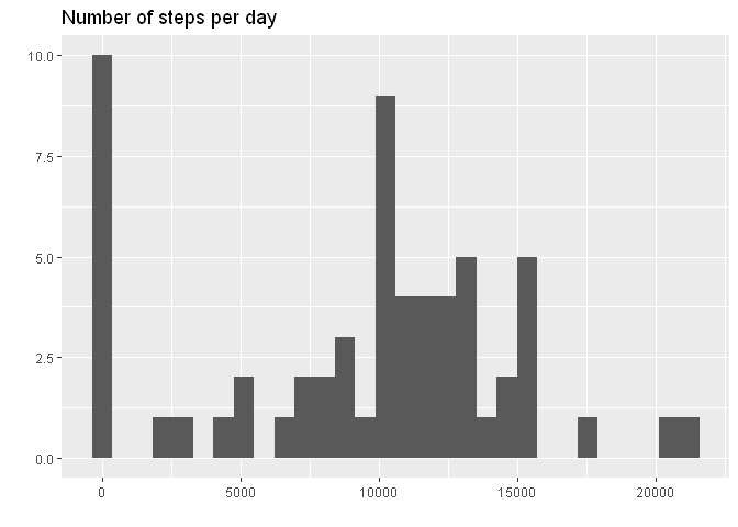
Repeating first steps of the assignement now with the imputed data. Summarizing the data:

total_steps_nna <- data_nna %>% group_by(date) %>%
  summarise(total = sum(steps))

g <- ggplot(total_steps_nna, aes(total))
g <- g + geom_histogram()
g <- g + labs(title="Number of steps per day", y="", x="")
g

## `stat_bin()` using `bins = 30`. Pick better value with `binwidth`.

mean_nna <- mean(total_steps_nna$total)
mean_nna

## [1] 10821.21

The mean total number of steps per day is: 10821.21 (was 9354.23 before imputation).

median_nna <- median(total_steps_nna$total)
median_nna

## [1] 11015

The median total number of steps per day is: 11015.00 (was 10395 before imputation).

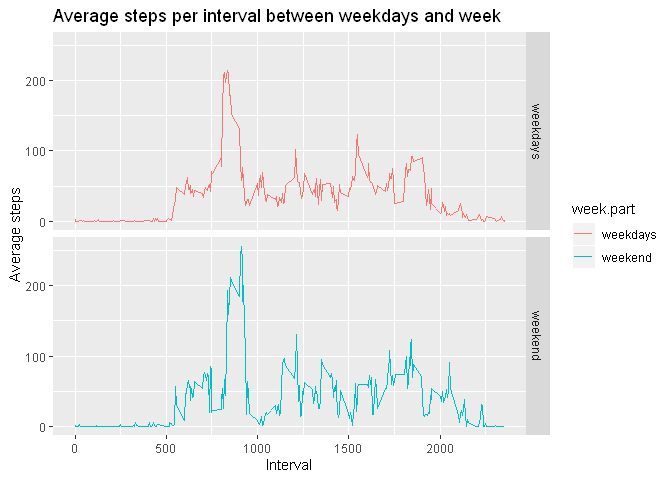
Are there differences in activity patterns between weekdays and weekends?

Summarizing the data:

steps_interval_nna <- data_nna %>% mutate(week.part = if_else(weekday %in% c(1,6), "weekend", "weekdays")) %>%
  group_by(week.part,interval) %>%
  summarise(mean = mean(steps, na.rm = TRUE))

g <- ggplot(steps_interval_nna, aes(interval, mean, col=week.part))
g <- g + geom_line()
g <- g + facet_grid(rows = vars(week.part))
g <- g + labs(title="Average steps per interval between weekdays and week", y="Average steps", x="Interval")
g