
EDA of NEI records of PM2.5
EDA of NEI records of PM2.5 for 1999, 2002, 2005, and 2008 (part of Exploratory Data Analysis by Johns Hopkins University)
This assignement focused only on plots as part of EDA. We did not checked for erroneous/missing data. Source code available on GitHub
Quick look at the data
NEI <- as_tibble(NEI)
SCC <- as_tibble(SCC)
str(NEI)
## Classes 'tbl_df', 'tbl' and 'data.frame':    6497651 obs. of  6 variables:
##  $ fips     : chr  "09001" "09001" "09001" "09001" ...
##  $ SCC      : chr  "10100401" "10100404" "10100501" "10200401" ...
##  $ Pollutant: chr  "PM25-PRI" "PM25-PRI" "PM25-PRI" "PM25-PRI" ...
##  $ Emissions: num  15.714 234.178 0.128 2.036 0.388 ...
##  $ type     : chr  "POINT" "POINT" "POINT" "POINT" ...
##  $ year     : int  1999 1999 1999 1999 1999 1999 1999 1999 1999 1999 ...
str(SCC)
## Classes 'tbl_df', 'tbl' and 'data.frame':    11717 obs. of  15 variables:
##  $ SCC                : Factor w/ 11717 levels "10100101","10100102",..: 1 2 3 4 5 6 7 8 9 10 ...
##  $ Data.Category      : Factor w/ 6 levels "Biogenic","Event",..: 6 6 6 6 6 6 6 6 6 6 ...
##  $ Short.Name         : Factor w/ 11238 levels "","2,4-D Salts and Esters Prod /Process Vents, 2,4-D Recovery: Filtration",..: 3283 3284 3293 3291 3290 3294 3295 3296 3292 3289 ...
##  $ EI.Sector          : Factor w/ 59 levels "Agriculture - Crops & Livestock Dust",..: 18 18 18 18 18 18 18 18 18 18 ...
##  $ Option.Group       : Factor w/ 25 levels "","C/I Kerosene",..: 1 1 1 1 1 1 1 1 1 1 ...
##  $ Option.Set         : Factor w/ 18 levels "","A","B","B1A",..: 1 1 1 1 1 1 1 1 1 1 ...
##  $ SCC.Level.One      : Factor w/ 17 levels "Brick Kilns",..: 3 3 3 3 3 3 3 3 3 3 ...
##  $ SCC.Level.Two      : Factor w/ 146 levels "","Agricultural Chemicals Production",..: 32 32 32 32 32 32 32 32 32 32 ...
##  $ SCC.Level.Three    : Factor w/ 1061 levels "","100% Biosolids (e.g., sewage sludge, manure, mixtures of these matls)",..: 88 88 156 156 156 156 156 156 156 156 ...
##  $ SCC.Level.Four     : Factor w/ 6084 levels "","(NH4)2 SO4 Acid Bath System and Evaporator",..: 4455 5583 4466 4458 1341 5246 5584 5983 4461 776 ...
##  $ Map.To             : num  NA NA NA NA NA NA NA NA NA NA ...
##  $ Last.Inventory.Year: int  NA NA NA NA NA NA NA NA NA NA ...
##  $ Created_Date       : Factor w/ 57 levels "","1/27/2000 0:00:00",..: 1 1 1 1 1 1 1 1 1 1 ...
##  $ Revised_Date       : Factor w/ 44 levels "","1/27/2000 0:00:00",..: 1 1 1 1 1 1 1 1 1 1 ...
##  $ Usage.Notes        : Factor w/ 21 levels ""," ","includes bleaching towers, washer hoods, filtrate tanks, vacuum pump exhausts",..: 1 1 1 1 1 1 1 1 1 1 ...
The NEI data is the amount of a specific Pollutant for a specific source SCC for a year in a county indicated by its FIPS code. The type represents the type of the emission sources as described here.
Let’s factorize the string values for NEI and check a summary of the NEI.
NEI$fips <- parse_factor(NEI$fips)
NEI$SCC <- parse_factor(NEI$SCC, levels = levels(SCC$SCC))
NEI$Pollutant <- parse_factor(NEI$Pollutant)
NEI$type <- parse_factor(NEI$type)
NEI$year <- parse_factor(as.character(NEI$year))
summary(NEI)
##       fips                 SCC             Pollutant
##  48201  :   9442   2275050011:  20301   PM25-PRI:6497651
##  06037  :   9320   2275070000:  16435
##  17031  :   7596   2275020000:  13926
##  06071  :   5710   2275050012:  12924
##  42003  :   5104   2265004010:  12881
##  06029  :   4970   2260004020:  12821
##  (Other):6455509   (Other)   :6408363
##    Emissions              type           year
##  Min.   :     0.0   POINT   : 516031   1999:1108469
##  1st Qu.:     0.0   NONPOINT: 473759   2002:1698677
##  Median :     0.0   ON-ROAD :3183599   2005:1713850
##  Mean   :     3.4   NON-ROAD:2324262   2008:1976655
##  3rd Qu.:     0.1
##  Max.   :646952.0
##
Similar summary for SCC.
summary(SCC)
##        SCC         Data.Category
##  10100101:    1   Biogenic:  82
##  10100102:    1   Event   :  71
##  10100201:    1   Nonpoint:2305
##  10100202:    1   Nonroad : 572
##  10100203:    1   Onroad  :1137
##  10100204:    1   Point   :7550
##  (Other) :11711
##                                                           Short.Name
##                                                                :   61
##  Paved Roads /unknown /unknown                                 :   12
##  Unpaved Roads /unknown /unknown                               :   12
##  Misc Manuf / Indus Processes /Other Not Classified            :   10
##  Marine Vessels, Military /unknown                             :    8
##  Pulp&Paper&Wood /Fugitive Emissions /Specify in Comments Field:    6
##  (Other)                                                       :11608
##                                               EI.Sector
##  Industrial Processes - Storage and Transfer       :1955
##  Industrial Processes - Chemical Manuf             :1702
##  Industrial Processes - NEC                        :1573
##  Solvent - Industrial Surface Coating & Solvent Use: 992
##  Mobile - On-Road Gasoline Light Duty Vehicles     : 518
##  Solvent - Degreasing                              : 390
##  (Other)                                           :4587
##                Option.Group     Option.Set
##                      :11450          :11436
##  P and P Product Tran:   44   B      :   84
##  Consumer/Commercial :   40   B1B    :   44
##  Commercial          :   30   B2B    :   37
##  Cattle              :   24   A      :   24
##  Poultry             :   20   B7B    :   19
##  (Other)             :  109   (Other):   73
##                            SCC.Level.One
##  Industrial Processes             :4787
##  Mobile Sources                   :1787
##  Petroleum and Solvent Evaporation:1563
##  Solvent Utilization              :1061
##  MACT Source Categories           : 686
##  Storage and Transport            : 489
##  (Other)                          :1344
##                      SCC.Level.Two
##  Chemical Manufacturing     :1264
##  Mineral Products           : 867
##  Highway Vehicles - Gasoline: 621
##  Organic Chemical Storage   : 605
##  Food and Agriculture       : 528
##  Highway Vehicles - Diesel  : 516
##  (Other)                    :7316
##                                                SCC.Level.Three
##  All Processes                                         :  168
##  Lawn and Garden Equipment                             :  143
##  Construction and Mining Equipment                     :  138
##  Heavy Duty Gasoline Vehicles 2B thru 8B & Buses (HDGV):  112
##  Light Duty Gasoline Trucks 1 & 2 (M6) = LDGT1 (M5)    :  112
##  Light Duty Gasoline Trucks 3 & 4 (M6) = LDGT2 (M5)    :  112
##  (Other)                                               :10932
##                   SCC.Level.Four      Map.To          Last.Inventory.Year
##  Other Not Classified    :  204   Min.   :2.020e+07   Min.   :1999
##  Total                   :  197   1st Qu.:3.040e+07   1st Qu.:1999
##  Total: All Solvent Types:  152   Median :3.079e+07   Median :2002
##  General                 :  114   Mean   :3.017e+08   Mean   :2002
##  Special Naphthas        :  106   3rd Qu.:4.030e+07   3rd Qu.:2005
##  Solvents: NEC           :   98   Max.   :2.805e+09   Max.   :2008
##  (Other)                 :10846   NA's   :11358       NA's   :8972
##              Created_Date             Revised_Date
##                    :9988                    :9090
##  2/13/2002 0:00:00 : 492   4/14/2003 0:00:00: 874
##  12/10/1999 0:00:00: 363   7/25/2008 0:00:00: 838
##  4/14/2009 0:00:00 : 166   7/27/2008 0:00:00: 272
##  10/19/2011 0:00:00:  62   2/13/2002 0:00:00:  95
##  4/15/2010 0:00:00 :  61   4/15/2010 0:00:00:  61
##  (Other)           : 585   (Other)          : 487
##                                                                                                                                                              Usage.Notes
##                                                                                                                                                                    :11693
##                                                                                                                                                                    :    5
##  includes bleaching towers, washer hoods, filtrate tanks, vacuum pump exhausts                                                                                     :    1
##  includes causticizer vents only or slaker and causticizer vents combined                                                                                          :    1
##  includes components within vacuum drum and non-vacuum drum systems including washer hoods, filtrate tank vents, and vacuum pump exhaust (some deckers and screens):    1
##  includes gases not in other low volume high concentration (LVHC) vent sources                                                                                     :    1
##  (Other)                                                                                                                                                           :   15
Some values seems missing. Quick overview.
summary(is.na(SCC))
##     SCC          Data.Category   Short.Name      EI.Sector
##  Mode :logical   Mode :logical   Mode :logical   Mode :logical
##  FALSE:11717     FALSE:11717     FALSE:11717     FALSE:11717
##
##  Option.Group    Option.Set      SCC.Level.One   SCC.Level.Two
##  Mode :logical   Mode :logical   Mode :logical   Mode :logical
##  FALSE:11717     FALSE:11717     FALSE:11717     FALSE:11717
##
##  SCC.Level.Three SCC.Level.Four    Map.To        Last.Inventory.Year
##  Mode :logical   Mode :logical   Mode :logical   Mode :logical
##  FALSE:11717     FALSE:11717     FALSE:359       FALSE:2745
##                                  TRUE :11358     TRUE :8972
##  Created_Date    Revised_Date    Usage.Notes
##  Mode :logical   Mode :logical   Mode :logical
##  FALSE:11717     FALSE:11717     FALSE:11717
##
Binding the two dataframes
data <- NEI %>%
  left_join(SCC, by = c("SCC" = "SCC"))
str(data)
## Classes 'tbl_df', 'tbl' and 'data.frame':    6497651 obs. of  20 variables:
##  $ fips               : Factor w/ 3263 levels "09001","09003",..: 1 1 1 1 1 1 1 1 1 1 ...
##  $ SCC                : Factor w/ 11717 levels "10100101","10100102",..: 31 32 35 113 121 124 125 186 190 193 ...
##  $ Pollutant          : Factor w/ 1 level "PM25-PRI": 1 1 1 1 1 1 1 1 1 1 ...
##  $ Emissions          : num  15.714 234.178 0.128 2.036 0.388 ...
##  $ type               : Factor w/ 4 levels "POINT","NONPOINT",..: 1 1 1 1 1 1 1 1 1 1 ...
##  $ year               : Factor w/ 4 levels "1999","2002",..: 1 1 1 1 1 1 1 1 1 1 ...
##  $ Data.Category      : Factor w/ 6 levels "Biogenic","Event",..: 6 6 6 6 6 6 6 6 6 6 ...
##  $ Short.Name         : Factor w/ 11238 levels "","2,4-D Salts and Esters Prod /Process Vents, 2,4-D Recovery: Filtration",..: 3339 3340 3300 3424 3391 3410 3408 3268 3247 3246 ...
##  $ EI.Sector          : Factor w/ 59 levels "Agriculture - Crops & Livestock Dust",..: 20 20 20 25 25 24 24 15 15 15 ...
##  $ Option.Group       : Factor w/ 25 levels "","C/I Kerosene",..: 1 1 1 1 1 1 1 1 1 1 ...
##  $ Option.Set         : Factor w/ 18 levels "","A","B","B1A",..: 1 1 1 1 1 1 1 1 1 1 ...
##  $ SCC.Level.One      : Factor w/ 17 levels "Brick Kilns",..: 3 3 3 3 3 3 3 3 3 3 ...
##  $ SCC.Level.Two      : Factor w/ 146 levels "","Agricultural Chemicals Production",..: 32 32 32 52 52 52 52 22 22 22 ...
##  $ SCC.Level.Three    : Factor w/ 1061 levels "","100% Biosolids (e.g., sewage sludge, manure, mixtures of these matls)",..: 886 886 317 886 317 692 692 886 317 317 ...
##  $ SCC.Level.Four     : Factor w/ 6084 levels "","(NH4)2 SO4 Acid Bath System and Evaporator",..: 2545 2546 2548 2544 2525 30 3 2544 2548 2525 ...
##  $ Map.To             : num  NA NA NA NA NA NA NA NA NA NA ...
##  $ Last.Inventory.Year: int  NA NA NA NA NA NA NA NA NA NA ...
##  $ Created_Date       : Factor w/ 57 levels "","1/27/2000 0:00:00",..: 1 1 1 1 1 1 1 1 1 1 ...
##  $ Revised_Date       : Factor w/ 44 levels "","1/27/2000 0:00:00",..: 1 1 1 1 1 1 1 1 1 1 ...
##  $ Usage.Notes        : Factor w/ 21 levels ""," ","includes bleaching towers, washer hoods, filtrate tanks, vacuum pump exhausts",..: 1 1 1 1 1 1 1 1 1 1 ...
Answering assignement’s questions with plots
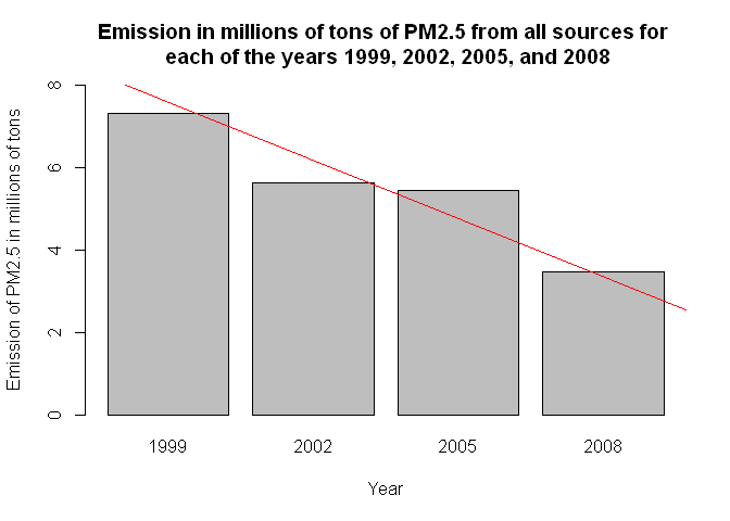
1. Have total emissions from PM2.5 decreased in the United States from 1999 to 2008?
Using base plotting system
totals <- data %>% group_by(year) %>%
  summarise(total = sum(Emissions)/10^6)
barplot(totals$total,
        names.arg = totals$year,
        main = "Emission in millions of tons of PM2.5 from all sources for \n each of the years 1999, 2002, 2005, and 2008",
        xlab = "Year",
        ylab = "Emission of PM2.5 in millions of tons",
        ylim = c(0,8))
abline(lm( totals$total ~as.numeric(totals$year)), col="red")
dev.print(device = png, file = "plot1.png", width = 500, pointsize=10)
## png
##   2
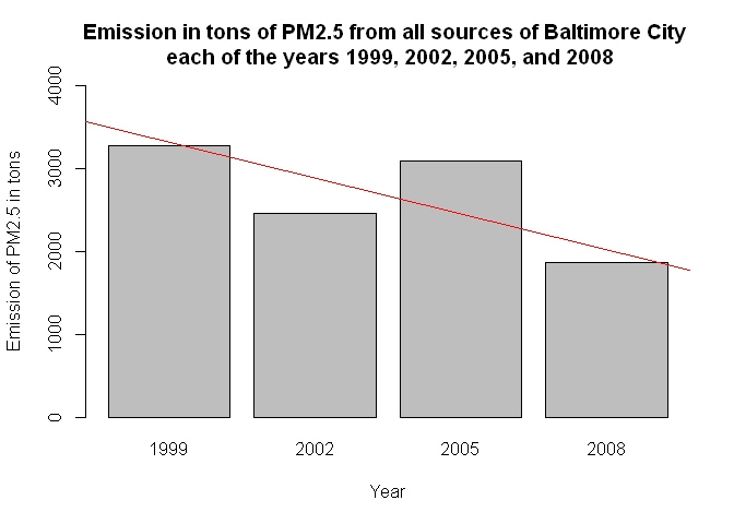
2. Have total emissions from PM2.5 decreased in the Baltimore City, Maryland (fips == “24510”) from 1999 to 2008?
Using base plotting system
totals_baltimore <- data %>% filter(fips == "24510") %>%
  group_by(year) %>%
  summarise(total = sum(Emissions))
barplot(totals_baltimore$total,
        names.arg = totals_baltimore$year,
        main = "Emission in tons of PM2.5 from all sources of Baltimore City \n each of the years 1999, 2002, 2005, and 2008",
        xlab = "Year",
        ylab = "Emission of PM2.5 in tons",
        ylim = (c(0,4000)))

abline(lm( totals_baltimore$total ~as.numeric(totals_baltimore$year)), col="red")
dev.print(device = png, file = "plot2.png", width = 500, pointsize=10)
## png
##   2
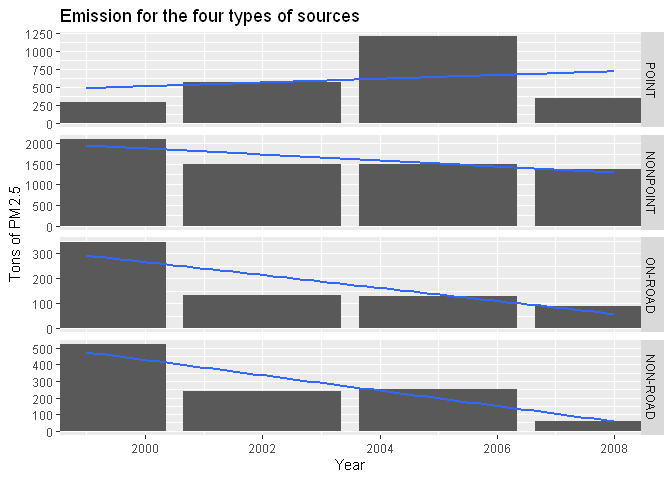
3. Of the four types of sources indicated by the type (point, nonpoint, onroad, nonroad) variable, which of these four sources have seen decreases in emissions from 1999–2008 for Baltimore City? Which have seen increases in emissions from 1999–2008?
Using ggplot2 plotting system
totals_baltimore_type <- data %>% filter(fips == "24510") %>%
  group_by(type, year) %>%
  summarise(total = sum(Emissions)) %>%
  mutate(year=as.numeric(levels(year))[year])
g<-ggplot(totals_baltimore_type) + geom_col(aes(x = year, y = total)) + geom_smooth(method = lm, aes(x = year, y = total), se = FALSE) + facet_grid(rows=vars(type), scales = "free_y")
g <- g + labs(x="Year", y ="Tons of PM2.5", title="Emission for the four types of sources")
g <- g + coord_cartesian(xlim=c(1999,2008))
print(g)
## Saving 7 x 5 in image
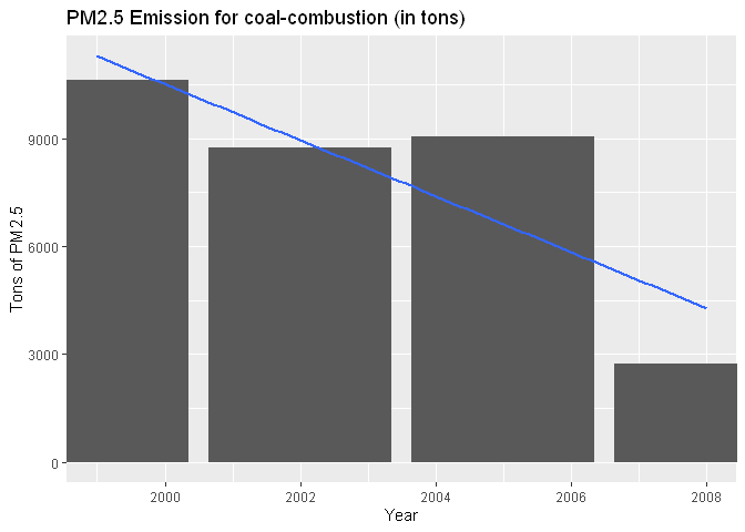
4. Across the United States, how have emissions from coal combustion-related sources changed from 1999–2008?
totals_coal <- data %>% filter(EI.Sector == "Fuel Comb - Comm/Institutional - Coal") %>%
  group_by(year) %>%
  summarise(total = sum(Emissions)) %>%
  mutate(year=as.numeric(levels(year))[year])
g <- ggplot(totals_coal) + geom_col(aes(x = year, y = total)) + geom_smooth(method = lm, aes(x = as.numeric(year), y = total), se = FALSE)
g <- g + labs(x="Year", y ="Tons of PM2.5", title="PM2.5 Emission for coal-combustion (in tons)")
g <- g + coord_cartesian(xlim=c(1999,2008))
print(g)
## Saving 7 x 5 in image
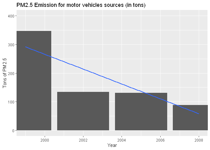
5. How have emissions from motor vehicle sources changed from 1999–2008 in Baltimore City?
- Hypothesis: We consider that those emissions are represented by the
- type onroad considering the information for
- epa.gov
- “NEI onroad sources include emissions from onroad vehicles that use gasoline, diesel, and other fuels”
totals_vehicle <- data %>% filter(type=="ON-ROAD", fips=="24510") %>%
  group_by(year) %>%
  summarise(total = sum(Emissions)) %>%
  mutate(year=as.numeric(levels(year))[year])
g <- ggplot(totals_vehicle) + geom_col(aes(x = year, y = total)) + geom_smooth(method = lm, aes(x = year, y = total), se = FALSE)
g <- g + labs(x="Year", y ="Tons of PM2.5", title="PM2.5 Emission for motor vehicles sources (in tons)")
g <- g + coord_cartesian(xlim=c(1999,2008),ylim=c(0,400))
print(g)
## Saving 7 x 5 in image
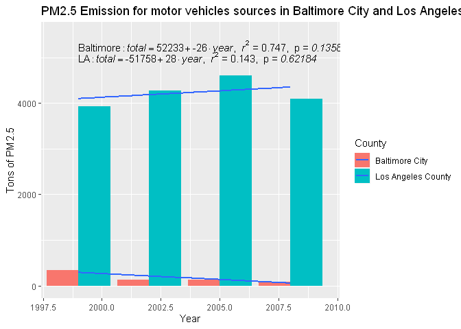
6. Compare emissions from motor vehicle sources in Baltimore City with emissions from motor vehicle sources in Los Angeles County, California fips==“06037”. Which city has seen greater changes over time in motor vehicle emissions?
totals_vehicle_comp <- data %>% filter(type=="ON-ROAD", fips=="24510" | fips=="06037") %>%
  group_by(fips,year) %>%
  summarise(total = sum(Emissions)) %>%
  mutate(year=as.numeric(levels(year))[year])
g <- ggplot(totals_vehicle_comp, aes(x = year, y = total, fill=fips))
g <- g + geom_col(position="dodge")
g <- g + geom_smooth(se = FALSE, method = lm)
g <- g + coord_cartesian(xlim=c(1998,2009.5),ylim=c(0,5500))
g <- g + geom_text(aes(x = 1999, y = 5250, hjust="left",label = paste("Baltimore: ", lm_eqn(totals_vehicle_comp %>% filter(fips=="24510"), "total", "year"))), parse = TRUE)
g <- g + geom_text(aes(x = 1999, y = 5000, hjust="left", label = paste("LA: ", lm_eqn(totals_vehicle_comp %>% filter(fips=="06037"), "total", "year"))), parse = TRUE)
g <- g + scale_fill_discrete(name="County", labels=c("Baltimore City", "Los Angeles County"), aesthetics = c("colour", "fill"))
g <- g + labs(x="Year", y ="Tons of PM2.5", title="PM2.5 Emission for motor vehicles sources in Baltimore City and Los Angeles County (in tons)")
print(g)
## Saving 7 x 5 in image